2 Statistical Software

In the past, researchers had to manually code all the statistical formulae for their analyses, which was tedious and error-prone. Today, statistical software simplifies this process dramatically. Researchers can shift their focus from the technical complexities of computation to understanding statistical logic and applying analyses correctly.

This section offers guidance on selecting appropriate statistical programming language, walks through the set-up process, and introduces the basics of conducting statistical analyses using modern tools.

2.1 Statistical software options:

R, Python, and Stata are the 3 most commonly used languages.

	R	Python	Stata
Cost	Free	Free	Requires License
IDE	RStudio/Posit	Many, Visual Code is good	Built in editor
Strengths	Best libraries for epidemiology, trial statistics.	Best libraries for text processing, machine learning, AI integration	Simple syntax; powerful quasi-experimental/meta-analysis packages. Used by U of U MSCI.
Weakness	Clunky syntax; many ‘dialects’	Overkill for many, complex development environment	Clunkiest machine learning, explainable programing, cost.
Explainable programmingWriting analytic code in a clear, structured, and understandable way so that readers (including reviewers, collaborators, and future researchers) can easily follow and replicate the steps of your analysis. In quantitative disciplines such as mathematics and computer science, providing such code is already standard practice. Medicine is beginning to adopt this approach, recognizing its importance for transparency and reproducibility.	Quarto	Jupyter, Quarto	Not native (though can use Jupyter)

There are a few other language options (SPSS, SAS, Julia, etc.), but they are omitted for brevity (generally, not the best modern options)

term	definition
Explainable programming	Writing analytic code in a clear, structured, and understandable way so that readers (including reviewers, collaborators, and future researchers) can easily follow and replicate the steps of your analysis. In quantitative disciplines such as mathematics and computer science, providing such code is already standard practice. Medicine is beginning to adopt this approach, recognizing its importance for transparency and reproducibility.

term

definition

Explainable programming

Writing analytic code in a clear, structured, and understandable way so that readers (including reviewers, collaborators, and future researchers) can easily follow and replicate the steps of your analysis. In quantitative disciplines such as mathematics and computer science, providing such code is already standard practice. Medicine is beginning to adopt this approach, recognizing its importance for transparency and reproducibility.

2.2 How to install

Choose the tab for the language(s) you plan to use:

2.2.1 Instructions:

1:	Install R Language	https://cran.r-project.org/	This installs the base programming language
2:	Install RStudio	https://posit.co/downloads/	RStudio is an IDEIntegrated Development Environment, a program that allows for writing, running, and debugging code within a single program. (integrated development environment) that allows you to write, execute, and debug code from within a single program.
3:	Install Quarto (formerly Markdown)	https://quarto.org/docs/get-started/	Facilitates sharing and explaining your code.

Install Python Language and dependencies

https://github.com/conda-forge/miniforge?tab=readme-ov-file

This (mini-forge) installs the base Python programming language, the things it depends on, and many useful packages

Create an environment

Execute the following commands in a terminal:

mamba create -n stats python=3.12 numpy pandas scipy statsmodels scikit-learn lifelines pingouinmatplotlib seaborn plotnine pyreadstatjupyterlab ipykernel jupytext –channel conda-forge

conda activate stats

This sets up an environment (controls the versions and packages that are used).

Install Visual Code

https://code.visualstudio.com/download

Visual Code is an IDE (integrated development environment) that allows you to write, execute, and debug code from within a single program.

*Note: there are many IDEIntegrated Development Environment, a program that allows for writing, running, and debugging code within a single program.. Visual Code is a classic one with a lot of functionality, though there are AI enabled ones (e.g. Cursor) that may be more helpful depending on how much programming you plan to do and whether you want to bother with the added complexity (discussed more in Section 2.7).

You can also use Quarto for explainable programming in Python - but Jupyter is a more common workflow so we focus on that.

1:	Get a product key	if U of U Trainee, contact me	This verifies you or your institutions’ purchase
2:	Install STATA	https://www.stata.com/install-guide/	Includes language and IDEIntegrated Development Environment, a program that allows for writing, running, and debugging code within a single program. (integrated development environment)

2.3 Packages

For common statistical analyses in any of these languages, specialized packages already exist that handle these tasks efficiently. Whenever you find yourself manually calculating or coding a statistical procedure, consider that someone likely has already written reliable, tested code that will perform the analysis faster and more accurately. You’ll want to use these packages whenever possible.

First, a few terms: functionA reusable piece of code that performs a specific task. Examples include calculating the mean of a dataset or running logistic regression., argumentsInputs provided to a function so it can perform its task. For instance, a function calculating a mean needs a dataset, while logistic regression requires data, the outcome variable, and predictor variables., packageA curated collection of functions designed to accomplish related tasks. Programming languages come pre-installed with basic packages, but you’ll often download additional packages to access specialized functions. Each language provides straightforward ways to locate and install new packages.

term	definition
arguments	Inputs provided to a function so it can perform its task. For instance, a function calculating a mean needs a dataset, while logistic regression requires data, the outcome variable, and predictor variables.
function	A reusable piece of code that performs a specific task. Examples include calculating the mean of a dataset or running logistic regression.
package	A curated collection of functions designed to accomplish related tasks. Programming languages come pre-installed with basic packages, but you’ll often download additional packages to access specialized functions. Each language provides straightforward ways to locate and install new packages.

2.3.1 Finding Packages

Where to find packages?	https://cran.r-project.org/web/views/
Command to install packages	`install.packages(```package_name```)`
How to access documentation file?	`?package_name` or `?command_name`

Where to find packages?	https://anaconda.org/conda-forge https://pypi.org/ https://github.com/topics/python
Command to install packages	`mamba install package_name` (rarely, packages that have not been compiled on conda-forge will require `pip install package_name` to be used)
How to access documentation file?	The project page on https://pypi.org/ or https://github.com/

Where to find packages?	`findit package_name`
Command to install packages	`ssc install package_name`
How to access documentation file?	`help package_name`

2.4 Reproducible Research

As mentioned before, Explainable programmingWriting analytic code in a clear, structured, and understandable way so that readers (including reviewers, collaborators, and future researchers) can easily follow and replicate the steps of your analysis. In quantitative disciplines such as mathematics and computer science, providing such code is already standard practice. Medicine is beginning to adopt this approach, recognizing its importance for transparency and reproducibility. is an increasingly important idea because programming errors frequently lead to erroneous research results. Understandable analytic code is important for co-authors to understand and verify what you’ve done, as well as facilitating replication and improvements.

Importantly (and, as will be discussed in Chapter 3), it’s not just the statistical design choices that can have an influence on the observed outcomes. Researchers must decide what data should be included, how the data should be cleaned, whether missing values will be imputed (and if so, how). All this occurs before talk of statistical tests, regressions, or presentation occur.

By some estimates, variation in how these pre-processing tasks are done accounts for more variability in findings than the design choices most readers focus on. Accordingly, the data processing code that is shared should include the entire process, from data cleaning to figure generation.

Statistical Methods and analysis: Pitfalls of research: https://journals.stfm.org/primer/2022/van-smeden-2022-0059/#.YvQyN_kxOPE.twitter How to structure the project files: https://medium.com/the-stata-guide/the-stata-workflow-guide-52418ce35006 Reproducible code info: https://twitter.com/lisadebruine/status/1504063177012695047?s=11 Citation for need to release analytic code: https://academic.oup.com/jamia/article-abstract/30/5/859/7056675

2.4.1 How to document and share code

In R, the easiest way to put together understandable and sharable code is to use Quarto documents (this website is actually is generated in Quarto).

Quarto creates notebooks that include segments that can contain text and pictures with other sections that contain executable R code. The segments containing R code can be executed in subsequent order - variables are shared between the boxes - thus allowing a long analytic pipeline to be broken up into small understandable chunks.

Tip

To create a new Quarto notebook, go to File->New->Quarto Document (*.qmd). Leave all the options in their default. Try it to make the below notebook.

For example, a hypothetical analysis might go something like:

2.4.1.1 Example Simulation of Coin Flips:

Our aim is to simulate the number of heads seen if a coin is flipped 50 times.

First, we create a function that simulates a fair coin flip: 50% probability heads (coded as 1), 50% probability of tails (coded as 0)

## one fair-coin flip: 1 = Heads, 0 = Tails
flip_coin <- function(n = 1) {
  sample(c(0, 1), size = n, replace = TRUE)
}

Then, we write a program that repesents a single simulation: the coin is flipped 50 times

## run one experiment of 50 flips and return #Heads
simulate_50 <- function() {
  sum(flip_coin(50))
}

## quick demo
set.seed(42)   # reproducible example
simulate_50()

[1] 27

Then, we perform 1000 simulations and store the results in an array, which we then present summary statistics on.

set.seed(42)                       # reproducible simulations
n_sims  <- 1000                    # how many experiments?
results <- replicate(n_sims, simulate_50())

summary(results)                   # five-number summary
hist(results,
     breaks = 20,
     main   = "Distribution of heads in 1 000 × 50-flip experiments",
     xlab   = "Number of heads")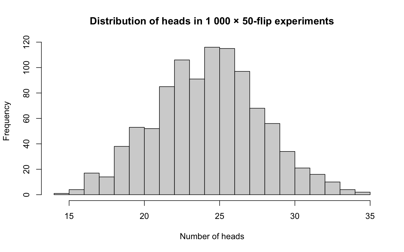

   Min. 1st Qu.  Median    Mean 3rd Qu.    Max. 
  14.00   22.00   25.00   24.74   27.00   35.00

2.4.1.2 Nuts and Bolts

Obviously, this example is a bit contrived, but is meant to show how the text and code can be interleaved to make the resulting output easy to understand. This quarto file can then be shared with collaborators (or posted on a code sharing site, such as github - provided none of the protected health information is hard coded into the text.

Tip

As an exercise, see if you can create your own Quarto markdown file, and extend the analysis to generate the interquartile range for the mean number of Heads in 50 flips.

In Python, the easiest way to put together understandable and sharable code is to use Jupyter notebooks.

Jupyter (like Quarto) creates notebooks that include segments that can contain text and pictures with other sections that contain executable Python code. The segments containing Python code can be executed in subsequent order - variables are shared between the boxes - thus allowing a long analytic pipeline to be broken up into small understandable chunks.

Tip

To create a new Jupyter notebook, go to File -> New Jupyter Notebook (*.ipynb). Try it to make the below notebook.

For example, a hypothetical analysis might go something like:

2.4.1.3 Example Simulation of 50 Coin Flips

Our aim is to simulate the number of heads seen if a coin is flipped 50 times.

First, we create a function that simulates a fair coin flip: 50% probability heads (coded as 1), 50% probability of tails (coded as 0)

import random

def flip_coin(n: int = 1) -> list[int]:
    """Return a list of 0 / 1 draws; 1 = heads, 0 = tails."""
    return random.choices([0, 1], k=n)

Then, we write a program that repesents a single simulation: the coin is flipped 50 times

def simulate_50() -> int:
    """Flip a coin 50 × and return the number of heads."""
    return sum(flip_coin(50))

random.seed(42)          # reproducible example
simulate_50()

Then, we perform 1000 simulations and store the results in an array, which we then present summary statistics on.

import numpy as np
import matplotlib.pyplot as plt

random.seed(42)

n_sims  = 1000
results = [simulate_50() for _ in range(n_sims)]

# summary statistics
print(f"min  : {min(results)}")
print(f"max  : {max(results)}")
print(f"mean : {np.mean(results):.2f}")
print(f"sd   : {np.std(results, ddof=1):.2f}")

# visualise
plt.hist(results, bins=20, edgecolor="black")
plt.title("Heads in 1 000 × 50-flip experiments")
plt.xlabel("Number of heads")
plt.ylabel("Frequency")
plt.show()

min  : 13
max  : 36
mean : 24.93
sd   : 3.48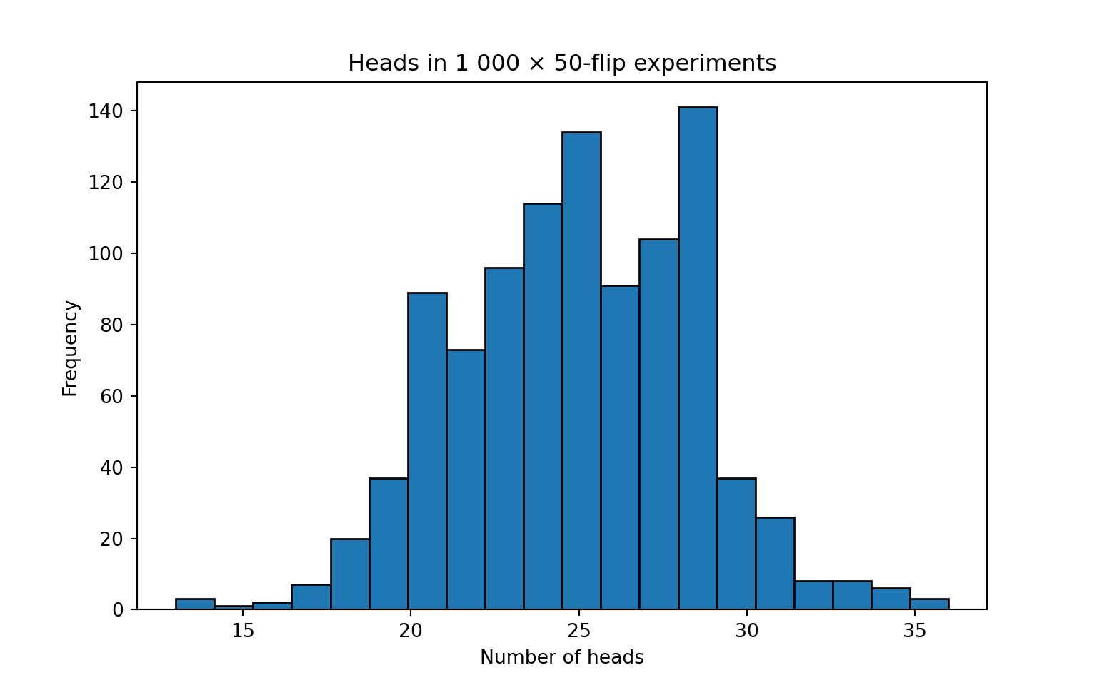

2.4.1.4 Nuts and Bolts

Obviously, this example is a bit contrived, but is meant to show how the text and code can be interleaved to make the resulting output easy to understand. This Jupyter notebook can then be shared with collaborators (or posted on a code sharing site, such as github - provided none of the protected health information is hard coded into the text.

Tip

As an exercise, see if you can create your own Jupyter notebook file, and extend the analysis to generate the interquartile range for the mean number of Heads in 50 flips.

Stata does not have a native notebook-style way to share code, but instead you have *.do files that contain a script of the relevant commands, and you can add comments using either # , *, or //* *//*

Tip

To create a new STATA do file, go to File -> New -> Do File (*.do). Try it to make the below script.

Stata Code: *.do files dont have an easy way to execute within the web page, so you’ll have to run the below script on your own machine to see the output.

*-----------------------------------------------------*
* 1.  Set the number of simulations                  *
*-----------------------------------------------------*
local nsims   = 1000      // how many experiments?
local nflips  = 50        // flips per experiment

set obs `nsims'           // create `nsims' empty observations

* Optional: reproducibility
set seed 42

*-----------------------------------------------------*
* 2.  Simulate 50 fair-coin flips for each experiment *
*     A "head" is coded 1 when runiform() < .5        *
*-----------------------------------------------------*
forvalues j = 1/`nflips' {
    generate byte flip`j' = runiform() < .5
}

*-----------------------------------------------------*
* 3.  Count heads in each experiment                  *
*-----------------------------------------------------*
egen heads = rowtotal(flip1-flip`nflips')

*-----------------------------------------------------*
* 4.  Inspect the sampling distribution               *
*-----------------------------------------------------*
summarize heads

histogram heads , ///
    width(1) start(0.5)          /// each bin spans one integer count
    title("Heads in `nsims' × `nflips'-flip experiments") ///
    xlabel(0(5)50)               /// tick every 5 heads; adjust as desired
    ylabel(, angle(horizontal))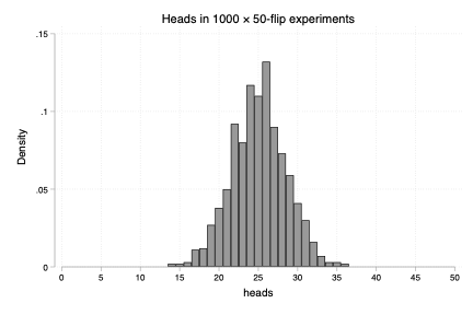

2.4.1.5 Nuts and Bolts

Obviously, this example is a bit contrived, but is meant to show how the text in comments and code can be interleaved to make the resulting output easy to understand. This do file can then be shared with collaborators (or posted on a code sharing site, such as github - provided none of the protected health information is hard coded into the text.

Tip

As an exercise, see if you can create your own Stata do file, and extend the analysis to generate the interquartile range for the mean number of Heads in 50 flips.

2.5 Reproducible Research

From a perspective of scientific rigor, sharing should also include the individual patient data to allow researchers to directly replicate or modify the reported analyses. However, despite research participant support for data sharing, privacy concerns and research ethics concerns generally do not permit the sharing of data, even if it has been pseudonomized. This is an active space where “ideal” and “actual” are far apart… but the current takeaway is that individual patient data should not ben shared unless that was explicitly part of the IRB authorization.

Further reading (R focus): https://raps-with-r.dev/intro.html building reproducible analytical pipelines: https://rap4mads.eu/?utm_source=substack&utm_medium=email Citation: reproducible computing: https://journals.plos.org/plosbiology/article?id=10.1371/journal.pbio.1001745

principles for reproducible and efficient computing; https://journals.plos.org/plosbiology/article?id=10.1371/journal.pbio.1001745

2.6 An Example: Meta-analyzing the effect of corticosteroids in CAP

Let’s use meta-analysis as a quick example of how to put this all into action.

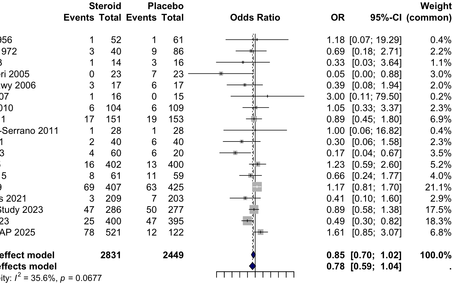
A meta-analysis typically accompanies a systematic review to comprehensively capture relevant studies on a question. Systematic reviews are complex, so we’ll skip the details here. Instead, we’ll perform a meta-analysis using a prepared spreadsheet of all known steroids-for-CAP studies (let me know if any studies are missing).

Download the data here: Steroid CAP Trials Spreadsheet

# ---- display the table ------------------------------------------------------
kable(steroids_pna, caption = "Steroids PNa meta-analysis data")

Steroids PNa meta-analysis data
study	year	chest_ma	int_death	int_alive	pla_death	pla_alive
Wagner	1956	0	1	51	1	60
McHardy	1972	0	3	37	9	77
Marik	1993	0	1	13	3	13
Confalonieri	2005	0	0	23	7	16
El Ghamrawy	2006	0	3	14	6	11
Mikami	2007	0	1	15	0	15
Snijders	2010	0	6	98	6	103
Melvis	2011	0	17	134	19	134
Ferrandez-Serrano	2011	0	1	27	1	27
Sabry	2011	0	2	38	6	34
Nafae	2013	0	4	56	6	14
Blum	2015	0	16	386	13	387
Torres	2015	0	8	53	11	48
Lloyd	2019	0	69	338	63	362
Wittermans	2021	0	3	206	7	196
ESCAPe Study	2023	0	47	239	50	227
Dequin	2023	0	25	375	47	348
REMAP-CAP	2025	1	78	443	12	110

Now, we’ll cover how you’d meta-analyze these studies in each language as an exercise:

2.6.1 Example Code

In R, here’s the steps needed to perform the meta-analysis:

First, set your working directory to wherever you downloaded the file. Then, we’ll need to make sure we have the right package to read in the spreadsheet

We’ll need the ‘readxl’ package to read in the *.xls file https://cran.r-project.org/web/packages/readxl/index.html

Then, we write code to import the spreadsheet with study data

library(readxl)                           # install.packages("readxl") if needed

## --- OPTION A – read from a local copy ------------------------------------
# setwd("~/your_dir")                       # uncomment and edit this line
# dat <- read_xls("Steroids PNa MA.xls", sheet = "Sheet1") |>
#        janitor::clean_names()

## --- OPTION B – read directly from the GitHub raw file             ----
url  <- "https://raw.githubusercontent.com/reblocke/statistics_sandbox/" |>
        paste0("1b87fb4e65da11a7f9541ea9c7f93b7e3947a13a/",
                "Steroids%20PNa/Steroids%20PNa%20MA.xls")

tmp  <- tempfile(fileext = ".xls")          # download to a temp file
download.file(url, tmp, mode = "wb")

dat  <- read_xls(tmp, sheet = "Sheet1") |>
        janitor::clean_names()                       # lower-case, snake_case

# Inspect the key columns
dat |>
  dplyr::select(study, year,
                int_death, int_alive,
                pla_death, pla_alive) |>
  print()

# A tibble: 18 × 6
   study              year int_death int_alive pla_death pla_alive
   <chr>             <dbl>     <dbl>     <dbl>     <dbl>     <dbl>
 1 Wagner             1956         1        51         1        60
 2 McHardy            1972         3        37         9        77
 3 Marik              1993         1        13         3        13
 4 Confalonieri       2005         0        23         7        16
 5 El Ghamrawy        2006         3        14         6        11
 6 Mikami             2007         1        15         0        15
 7 Snijders           2010         6        98         6       103
 8 Melvis             2011        17       134        19       134
 9 Ferrandez-Serrano  2011         1        27         1        27
10 Sabry              2011         2        38         6        34
11 Nafae              2013         4        56         6        14
12 Blum               2015        16       386        13       387
13 Torres             2015         8        53        11        48
14 Lloyd              2019        69       338        63       362
15 Wittermans         2021         3       206         7       196
16 ESCAPe Study       2023        47       239        50       227
17 Dequin             2023        25       375        47       348
18 REMAP-CAP          2025        78       443        12       110

Next, we’ll need to get a package to do the meta-analysis. Here’s a list of relevant packages: https://cran.r-project.org/web/views/MetaAnalysis.html

The ‘meta’ package looks good. Try using `install.packages(‘meta’)` to install it, then you can you can access the documentation using `?meta`

Now, we’ll perform a random-effects meta-analysis (Using DL variance stimator)

library(meta)                             # install.packages("meta")

Loading required package: metadat

Loading 'meta' package (version 8.1-0).
Type 'help(meta)' for a brief overview.

m <- metabin(
  event.e     = int_death,
  n.e         = int_death + int_alive,
  event.c     = pla_death,
  n.c         = pla_death + pla_alive,
  studlab     = paste(study, year),
  data        = dat,
  sm          = "OR",      # odds ratio
  method.tau  = "DL",      # <-- DerSimonian–Laird estimator
  method.random.ci        = FALSE
)

Lastly, we’ll need to plot the result as a Forest Plot on a log scale (always log scale with ratio variables)

forest(
  m,
  comb.fixed  = FALSE,
  comb.random = TRUE,
  print.tau2  = FALSE,
  backtransf  = TRUE,
  xlab        = "Odds Ratio (death)",
  leftlabs    = c("Study (year)", "Steroid", "Placebo"),
  xlog        = TRUE,
  at          = c(1/32, 1/16, 1/8, 1/4, 1/2, 1, 2, 4, 8, 16, 32),
  label.e     = "Steroid",
  label.c     = "Placebo",
  col.diamond = "navy",
  overall.lty = 2,
  ## keep the default right-hand columns
  # rightcols = FALSE,          # <-- delete this line
  main        = "Steroids OR for Death, Random-Effects Meta-analysis"
)

In Python, here’s the steps needed to perform the meta-analysis:

First, set your working directory to wherever you downloaded the file. Then, we’ll need to make sure we have the right package to read in the spreadsheet

Then, we write code to import the spreadsheet with study data using pandas

import pandas as pd

# --- OPTION A: read directly from disk -------------------------------
# df = pd.read_excel("Steroids PNa MA.xls", sheet_name="Sheet1")

# --- OPTION B:  For this demo we fetch the raw file from GitHub (same content as R block)
url = ("https://raw.githubusercontent.com/reblocke/statistics_sandbox/"
       "1b87fb4e65da11a7f9541ea9c7f93b7e3947a13a/"
       "Steroids%20PNa/Steroids%20PNa%20MA.xls")
df = pd.read_excel(url)           # GitHub serves raw file

# clean column names to snake_case like janitor::clean_names()
df.columns = (df.columns
                .str.strip()
                .str.lower()
                .str.replace(" ", "_"))

# quick sanity check
df.head(18)

                study  year  chest_ma  ...  int_alive  pla_death  pla_alive
0              Wagner  1956         0  ...         51          1         60
1             McHardy  1972         0  ...         37          9         77
2               Marik  1993         0  ...         13          3         13
3        Confalonieri  2005         0  ...         23          7         16
4         El Ghamrawy  2006         0  ...         14          6         11
5              Mikami  2007         0  ...         15          0         15
6            Snijders  2010         0  ...         98          6        103
7              Melvis  2011         0  ...        134         19        134
8   Ferrandez-Serrano  2011         0  ...         27          1         27
9               Sabry  2011         0  ...         38          6         34
10              Nafae  2013         0  ...         56          6         14
11               Blum  2015         0  ...        386         13        387
12             Torres  2015         0  ...         53         11         48
13              Lloyd  2019         0  ...        338         63        362
14         Wittermans  2021         0  ...        206          7        196
15       ESCAPe Study  2023         0  ...        239         50        227
16             Dequin  2023         0  ...        375         47        348
17          REMAP-CAP  2025         1  ...        443         12        110

[18 rows x 7 columns]

Next, we’ll need to get a package to do the meta-analysis. We’ll use the statsmodels (statsmodels.stats.meta_analysis) package https://www.statsmodels.org/dev/examples/notebooks/generated/metaanalysis1.html

Now, we’ll perform a random-effects meta-analysis (Using DL variance estimator - which takes some manual preparation work).

import numpy as np
from statsmodels.stats.meta_analysis import (
    effectsize_2proportions,    # log-odds-ratio + variance   
    combine_effects             # pooling with DL            
)

# --- 2. per-study log(OR) & variance with 0.5 correction --------------------
a = df["int_death"].to_numpy(dtype=float)
b = df["int_alive"].to_numpy(dtype=float)
c = df["pla_death"].to_numpy(dtype=float)
d = df["pla_alive"].to_numpy(dtype=float)

# continuity correction if any cell is zero in that study
cc = ((a == 0) | (b == 0) | (c == 0) | (d == 0)).astype(float) * 0.5
a += cc; b += cc; c += cc; d += cc

log_or = np.log((a * d) / (b * c))
var_or = 1 / a + 1 / b + 1 / c + 1 / d          # variance of log(OR)

# --- 3. DerSimonian-Laird random-effects pooling ---------------------------
res = combine_effects(log_or, var_or, method_re="dl")   # DL estimator

print("Current statsmodels version:", importlib.metadata.version("statsmodels"))

sf = res.summary_frame()          # still log-OR
sf["eff"]    = np.exp(sf["eff"])
sf["ci_low"] = np.exp(sf["ci_low"])
sf["ci_upp"] = np.exp(sf["ci_upp"])
print(sf.round(3))

Current statsmodels version: 0.14.4
                     eff  sd_eff  ci_low  ci_upp   w_fe   w_re
0                  1.176   1.427   0.072  19.285  0.005  0.010
1                  0.694   0.696   0.177   2.714  0.020  0.036
2                  0.333   1.219   0.031   3.638  0.006  0.013
3                  0.047   1.495   0.002   0.878  0.004  0.009
4                  0.393   0.814   0.080   1.936  0.014  0.028
5                  3.000   1.672   0.113  79.499  0.003  0.007
6                  1.051   0.594   0.328   3.369  0.027  0.046
7                  0.895   0.356   0.446   1.796  0.075  0.092
8                  1.000   1.440   0.059  16.822  0.005  0.010
9                  0.298   0.850   0.056   1.578  0.013  0.026
10                 0.167   0.711   0.041   0.672  0.019  0.035
11                 1.234   0.380   0.586   2.600  0.066  0.085
12                 0.659   0.506   0.245   1.774  0.037  0.059
13                 1.173   0.190   0.808   1.702  0.264  0.150
14                 0.408   0.697   0.104   1.599  0.020  0.036
15                 0.893   0.223   0.576   1.383  0.191  0.137
16                 0.494   0.258   0.297   0.819  0.142  0.123
17                 1.614   0.328   0.849   3.069  0.089  0.100
fixed effect       0.861   0.098   0.711   1.042  1.000    NaN
random effect      0.785   0.145   0.590   1.044    NaN  1.000
fixed effect wls   0.861   0.121   0.678   1.092  1.000    NaN
random effect wls  0.785   0.146   0.590   1.045    NaN  1.000

Lastly, we’ll need to plot the result as a Forest Plot on a log scale (always log scale with ratio variables)

import matplotlib.pyplot as plt

# draw the default forest plot (no extra kwargs)
fig = res.plot_forest(use_exp=True)

# post-process the axis with Matplotlib
ax = fig.axes[0]          # the single Axes returned by plot_forest
ax.set_xscale("log")
ax.set_xlim(0.03125, 32)
ax.set_xlabel("Odds Ratio (death)")
ax.set_xticks([1/32, 1/16, 1/8, 1/4, 1/2, 1, 2, 4, 8, 16, 32])
ax.set_xticklabels(
    ["1/32", "1/16", "1/8", "1/4", "1/2",
     "1", "2", "4", "8", "16", "32"]
)

plt.title("Steroids OR for Death, Random-Effects Meta-analysis (DL)")
plt.tight_layout()
plt.show()

(0.03125, 32)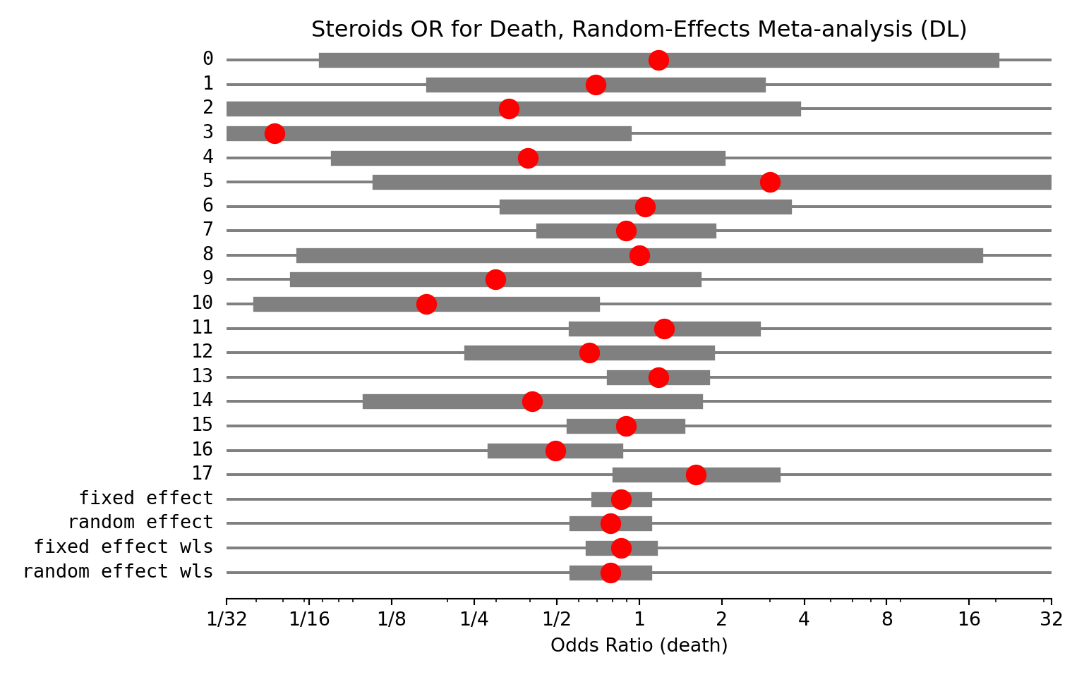

As before, Stata does not have a native notebook-style way to execute code within this webpage, so you’ll have to run the below script on your own machine to see the output.

Here’s the steps:


*-----------------------------------------------------*
* 1. Set your_dir to wherever you downloaded the doc  *
*-----------------------------------------------------*
cd your_dir

*-----------------------------------------------------*
* 2. Import the Spreadsheet with Study Data           *
*-----------------------------------------------------*
clear
import excel "Steroids PNa MA.xls", sheet("Sheet1") firstrow case(lower)
list study year int_death int_alive pla_death pla_alive
label variable study "Study"

*-----------------------------------------------------*
* 3. Meta-analyze the studies using REML              *
*-----------------------------------------------------*
meta esize int_death int_alive pla_death pla_alive, random(reml) esize(lnor) studylabel(study year) 

*-----------------------------------------------------*
* 4. Create a forest plot with the result             *
*-----------------------------------------------------*
meta forestplot, eform  nullrefline(lcolor(gs3)) esrefline(lcolor(gs3) lpattern(dash_dot)) title("Steroids OR for Death, Random-Effects Meta-analysis")  xsize(11) ysize(7) xscale(log range(0.01 64)) xlabel(0.03125 "1/32" 0.0625 "1/16" 0.125 "1/8" 0.25 "1/4" 0.5 "1/2" 1 "1" 2 "2" 4 "4" 8 "8" 16 "16" 32 "32")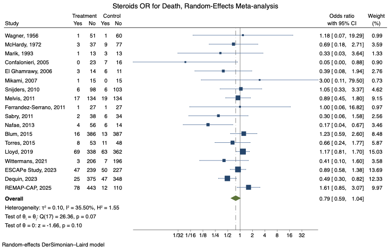

2.7 Large Language Models (LLMs)

Randomized trials (!) show the professional coders are more productive when using LLMs to assist with code. Novices see larger relative gains because LLMs supply boiler-plate, interface syntax, and “first drafts” of code.

However, LLMs can hallucinate. They can also be tricky to use. Here’s some guidance that holds for any of the frontier company models (OpenAI: chatGPT, Anthropic Claude, Google Gemini)

2.7.1 Minimal viable set up:

Step	Why	Tool
Use your local IDEIntegrated Development Environment, a program that allows for writing, running, and debugging code within a single program. with a plain chat tab or desktop app.	Allows you to (quality)control inputs and outputs - which is harder to do with an integrated IDE (e.g. Cursor) or agentic models.	Built-in browser tab or official desktop app
Do NOT upload data to LLMs	The companies do not have Business Access Agreements with institutions, and this generally violates the consent/IRB authorization of most studies.	Keep data local, only share schemas (descriptions of the variables) or mock data.
Sanity test all LLM-generated code	Hallucinations exist, and often task specifications are subtly wrong	You can writing coding tests (so called “Unit Tests”, but should also visualize and consider all code (this is true when not using LLMs)
Give the LLM examples of what you want	LLMs are VERY good at understanding what existing code does - and can often modify much better than create de-novo	Use things like: here’s the code that generates this figure - modify it so that title is larger.
Give the LLM specific instructions, often with steps	The more “context” you give the LLM for what you want, the more likely the associations it follows will be relevant	Detailed instructions in the prompt. More on prompt engineering is available here: https://docs.anthropic.com/en/docs/build-with-claude/prompt-engineering/overview

Important

Never put PHI into a commercial LLM interface. Not even ‘publicly available’ data like MIMIC (which has terms of use that forbid this). Most companies market their LLMs as being able to act as data-analysts on your behalf (meaning, you give it the data and it analyzes it for you). Don’t do this. https://pmc.ncbi.nlm.nih.gov/articles/PMC10937180/

Instead, use the LLM to help you write statistical code that you then run on your machine.

Mistake	Consequence	Quick fix
Skipping LLM entirely	Slower learning curve	Use it for boiler-plate, explaining things, first drafts
Blind trust	Silent bugs ≈ misleading science	Unit tests, peer-review, benchmark against known outputs
Vague prompt	Generic, unusable code	Include language, package, data schema, desired output
Manual debugging	Time sink	Feed the exact error message back to the model
Pasting PHI	Compliance breach	Use synthetic or sampled data; keep true identifiers offline

2.8 Local (and other) resources

One Data Science Hub Workshops: https://utah-data-science-hub.github.io/education_archived.html
Request CTSI help: https://ctsi.utah.edu/cores-and-services/triad
R book (very good, but in-depth): https://r4ds.had.co.nz/index.html

Guide to Python for those familiar with STATA - https://github.com/aeturrell/coding-for-economists/blob/main/coming-from-stata.md Guide to Python for those familiar with R - https://www.emilyriederer.com/post/py-rgo/?utm_source=substack&utm_medium=email

TODO List:

# find citation on how frequently errors occur in scientific programming.  - https://www.nature.com/collections/prbfkwmwvz 
# find citation for data cleaning influence on stability of findings